Real-time System Identification
2016-08-12 00:00:00 +0000
Overview
The Neurobionics Lab at the Rehabilitation Institute of Chicago aims to advance human mobility through an improved understanding of how the brain controls joint dynamics during tasks such as locomotion. The goal of this project was to identify system parameters of joint dynamics in real time, with the aim to study how people control the dynamics of their joints during tasks. Understanding how people control their movement will improve wearable robotic technologies by incorporating how people naturally move and interact with their environment.
We quantify neuromuscular control of ankle dynamics by estimating parameters of an equivalent mechanical system, namely inertia, stiffness, and damping. These parameters define how the system torque output will relate to the position input and describe a linear, time-varying, second-order system. This project explores the limits of real-time parameter identification using system identification techniques in signal processing and optimization on a Simulink model of the system. Identification is analyzed for how well the estimated parameters match the actual parameters and how well the estimated system explains the behavior of the actual system. Results are promising for identification in .3 seconds for a signal with up to 10% added noise, even if system parameters change up to 150% over the course of identification.
This implementation relies on work from the following sources:
Silvia, Manuel T., and Enders A. Robinson. 1978. Deconvolution of geophysical time series in the exploration for oil and natural gas. Amsterdam: Elsevier Scientific Pub. Co.
Keesman, Karel J. System identification: an introduction. Springer Science & Business Media, 2011.
Kearney, Robert E., and Ian W. Hunter. “System identification of human joint dynamics.” Critical reviews in biomedical engineering 18, no. 1 (1989): 55-87.
Mooney, Luke M., Stephanie L. Ku, Madeleine Abromowitz, Jacob A. Mooney, Xu Sun, and Qifang Bao. “Measuring muscle stiffness by linear mechanical perturbation.” In 2015 IEEE 12th International Conference on Wearable and Implantable Body Sensor Networks (BSN), pp. 1-5. IEEE, 2015.
Introduction
With a position input and a torque output, deconvolution is performed to the input-output cross correlation and the input autocorrelation to find the system impulse response. A second order system is fit to this response in the frequency domain, and variance accounted for (VAF) is used as a measure of correctness. VAF was explored for varying levels of noise, window length, and changing system dynamics.
Simulink model
In the following analysis, a Simulink model of a linear time-varying second order system was used to model joint impedance and analyze the effect of various parameters on identification.

The bulk of the signal blocks in the diagram model an LTV second order mass spring damper system and its equivalent transfer function:
where I is inertia, B is damping, and K is stiffness (inertia is used instead of mass). K varies according to a sine wave of which the amplitude, frequency, and bias can be set. The transfer function block models the same system with no varying parameters for model correctness verification.
Input
The reliability of the estimate of joint dynamics depends on the relative magnitudes of the input signal and noise. The best practice is for the input waveform to contain significant power over the range of frequencies for which the system is expected to respond. In this analysis, two input waveforms were tested: pseudo-random binary sequence (PRBS) and filtered Gaussian white noise distribution.
PRBS is generated by the equation , where u is the input, w(t) is a computer-generated white noise process, and p0 is the switching probability of value 0.5 in this analysis.
Gaussian white noise input is created with the matlab command randn, which generates a zero-mean normal distribution of random numbers. This input is then low-pass filtered at 200Hz to remove high frequency information.

Simulation
The Gaussian white noise input is scaled to an amplitude of ± 0.05 rad and used to stimulate the system model; torque output is recorded. Noise is added to the output data to more accurately simulate a real system; the signal to noise ratio examined was between 10 and higher. Data is examined in windows of time; windows of length 100ms through 1 sec were analyzed.
While the ultimate analysis used a continuous input, using pulses of input to the system was also tested. Due to the nature of convolution, a stimulated system will not come fully to rest until some amount of time has passed since the stimulation ceased. For example, a system with an impulse response of 1 second that receives 1 second of input will not come fully to rest until 2 seconds have passed. Therefore, using a window of time from a continuous input to a system does not fully capture the system response as we have not allowed the system to come to rest, adding noise to the deconvolution. Since the system in question has impulse responses that last only about 30ms and we do not expect joint impedance to be changing faster than 10Hz, using an input pulse of 50ms and then zero input for 50ms should allow us to fully solve the deconvolution without adding noise from incomplete system response.
While the method of input pulses is more mathematically sound in terms of complete information for deconvolution, the short segments were ultimately not as capable of handling noise as longer windows of continuous input despite their lack of complete response. Therefore we do not pursue pulse input further.
Deconvolution
While the impulse response of a perfect system can be found by sequentially solving for the relationship between the input and output data, in practice the presence of any noise completely distorts this solution. An alternative method is to use the auto- and cross-correlations to reconstruct the unit-impulse response using the Wiener-Hopf equation where ruy is the cross-correlation between the input and output data, ruu is the auto-correlation of the input data, g(k) is the impulse response we are looking for, and l is the lag. These correlations reduce the impact of noise since noise is uncorrelated with itself. Substituting the input and output data values into the Wiener-Hopf equation for a certain duration of time and rewriting the results in matrix form gives an equation where the cross-correlation is equivalent to the Toeplitz matrix of the auto-correlation multiplied by the impulse response. If the matrix is invertible, the impulse response can be directly found. A faster method than matrix inversion exploits the symmetric properties of the Toeplitz matrix in Toeplitz recursion, developed by Wiggins and Robinson in 1965 (referred to as the EUREKA method by Silvia and Robinson). This scheme solves for filter coefficients (in this case the impulse response) using the prediction-error variance and is faster than matrix inversion for the array lengths we are looking for. The table below shows the time taken to solve for impulse response using the two methods as a function of various array lengths. The time shown is the average of 10 trials. We are using arrays lengths of 300 – 1500, so the Eureka method is much faster.
| Array length | 100 | 200 | 400 | 800 | 1600 | 3200 | 6400 | 12800 |
|---|---|---|---|---|---|---|---|---|
| Eureka | .001 sec | .002 | .006 | .015 | .04 | .128 | .50 | 2.17 |
| Inversion | .0005 sec | .001 | .007 | .028 | .12 | .543 | 2.4 | 15.8 |
In addition, here the noisy output is also low-pass filtered with a cutoff frequency of 100Hz before the cross-correlation is calculated. In theory this step should be unnecessary but was found to perform better in simulation.

Parameterization
Once the impulse response has been identified, we want to parameterize it to fit a second order system and estimate the parameters for inertia, damping, and stiffness. This fitting is performed using the Matlab command fminsearch, which performs a multidimensional unconstrained nonlinear minimization. The search is optimized over the three parameters and minimizes the error between the estimated system and the solved system response in the frequency domain. To convert to the frequency domain, a finite Fourier transform is applied to the impulse response; the frequency response function is the absolute value of the first half of this transform. The frequency resolution is 1 over the time length of the impulse response. The frequency response of the estimated system is found by mapping the transfer function to the complex plane (s → jw) over the desired frequency range. The frequency responses are compared using a log fit to deemphasize the contribution of inertia to the fit. The process of impulse response identification and parameterization takes a total of around .065 seconds.

Error testing
For a given transfer function, the error in parametrization was examined as a function of window length (for input-output data) and signal to noise ratio (with noise as a percentage of signal). Error is consistently below 10% for damping and stiffness estimates with a window length of at least 300ms regardless of noise level. Inertia estimates are inconsistent throughout.

For a transfer function with constant values for inertia and damping and a window length of 300ms, variance accounted for (VAF) was examined as a function of impedance change and noise. Changing impedance was modeled by using a stiffness parameter that monotonically increased from its start value to as large as 148% of its start value over the course of the window length. The graph below shows variance unaccounted for (1 minus VAF). The variance stays low throughout any impedance change, and grows with noise.

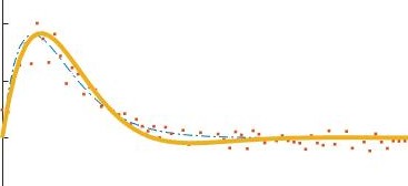
The parameter estimation over time was looked at for various frequencies of stiffness change for a sense of how fast the parameters can change and still achieve reasonable estimation. Two examples are shown below.


Preliminary results
Data collected by Tim Reissman in an experiment measuring joint impedance was examined. In this experiment, the right ankle was strapped to a motor and perturbed around a stationary position. The position input was filtered Gaussian white noise input with an amplitude of 0.035 rad, 5 Hz cutoff frequency, and a total time of 65 seconds. Position and torque information were collected at a sampling rate of 2500Hz. Data was also recorded for the machine without a person attached to estimate the contribution of the machine to the output and be able to remove this baseline torque.
The machine is modeled as a mapping from acceleration to torque. To use acceleration, a five point differentiation of the position data was performed twice, but the slight noise in the recorded data made this differentiation very noisy. Instead, the MATLAB command diff was used, then low-pass filtered with a cutoff frequency of 10Hz at each differentiation. The impulse response of the machine dynamics was estimated using the first 8 seconds of data. For the most accurate result, the entire 65 second recording period would be used, but this proved time-prohibitive in this analysis.

This impulse response was used to predict the torque response of the machine to the filtered Gaussian white noise input as acceleration and to a PRBS input as acceleration. The VAF for the PRBS input was 90.04% and the VAF for the FWGS was 89.32%. In comparison, the impulse response from position to torque was also used to predict the torque response of the machine. With this mapping, the VAF for the PRBS input was 22% and the VAF for the FGWN input was 58%.

This identified impulse response is used to identify the machine contribution to the data by convolving the acceleration with the machine impulse response and subtracting out this contributed torque. The residual torque is used to find the impulse response and parametrized system for the ankle in .3 second windows with position as the input.
The results over the length of the data are shown below, with the top three plots showing parameter values, and the fourth plot showing variance accounted for between the impulse response and the parameterized response. The preliminary results of this analysis of real data do not do a satisfactory job of parameter estimation. The values estimated for inertia, damping, and stiffness are not at all consistent and the variance accounted for is very low. One possible source of error is the low frequency of the input (cutoff frequency of 10Hz versus a cutoff frequency of 200Hz in simulation testing). Other sources of error include the presence of a large amount of noise and an initial guess for the parameter estimation that has great influence on the predicted value. The parameter values are also highly dependent on the cutoff frequency used for the fit estimation. Further work is needed to examine the identification of real data.

Conclusion
This project explored the limits of real-time system identification. It has shown that parameter estimation is possible with less than 10% error for a window length of .3 seconds or greater with up to 10% signal to noise ratio. Variance accounted for remains above 90% until approximately 6% signal to noise ratio with up to a 150% change in impedance. These results are promising for understanding how people control the stiffness of their ankles during tasks. In the future, these results can be extended to experimental data and used to parameterize ankle impedance in real time.